Google Sheets has turned out to be an effective way of how we create excel sheets online without any hassle. The platform has made it easier for the users to keep track of data and maintain it with ease on a regular basis. Ever since the introduction, Google Sheets has been used by several people, including huge organizations across the world.
Google Sheets has a lot of features, and one of the essential ones is freezing or unfreezing rows. When working on a big Google spreadsheet, it becomes essential for us to keep some of the rows and columns in the view. Suppose you want to see a particular row even after scrolling down the sheet. This is where freezing or unfreezing rows come in handy. Now, if you want to know how to do the same, then keep reading.
Also Read
Freezing or Unfreezing Rows in Google Sheets
The process of freezing or unfreezing rows in Google Sheets is a straightforward method. Here’s how you can do it:
Freezing Rows in Google Sheets
- Open Google Sheets and select the row you want to freeze.

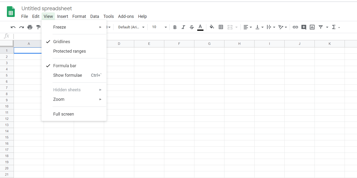
- Click on View from the top bar.
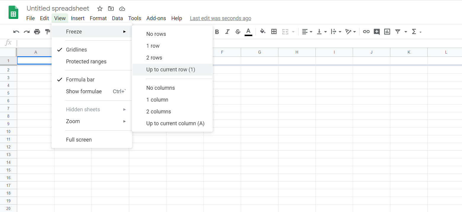
- Now tap on Freeze rows and select the preferred option.

Once you have selected the option, you will notice that row you have selected will freeze no matter where you go on the Google Sheet.
Unfreezing Rows in Google Sheets
- Once you are inside Google Sheets, select the row you want to unfreeze.
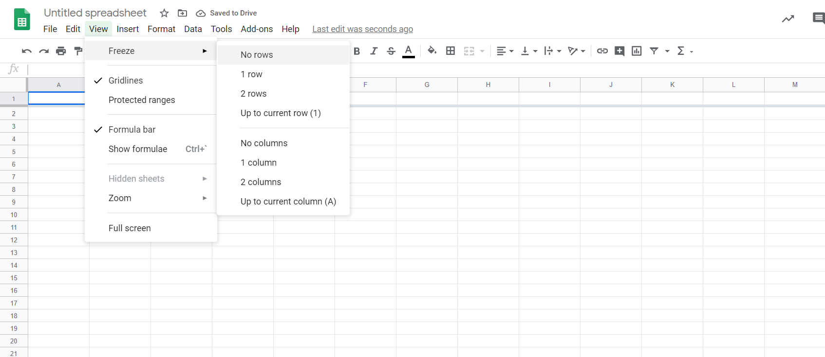
- Tap on View and select Freeze rows.

- From the options, select No rows option.
That’s it, folks. This is the simplest way you can freeze or unfreeze rows in Google Sheets. I hope you can manage the Google Sheets more effectively using this method.