Google Sheets is one of the best free alternatives to Microsoft’s Office suite of applications. It comes with most features that one will need from a spreadsheet application. Creating and managing spreadsheets using this web-based spreadsheet tool is just as easy as using any other offline/online software. Moreover, Google Sheets offers one useful feature that is known as Pivot Tables.
In this post, we will take a look at the Pivot Table in Google Sheets and talk about how and where to use it. Thankfully, understanding the Pivot Table in Google Sheets does not require much time. And you’ll be able to make use of this powerful tool within no time at all. First off, let’s understand what is a Pivot Table before diving into how to use it.
Also Read

What is a Pivot Table in Google Sheets?
A Pivot Table lets you analyze large sums of data in an organized manner. Moreover, it does away with the need to enter different codes and functions to get the desired results. The Pivot Table basically lets you select columns and rows that you want to analyze and summarise.
Then, it creates an easy to understand table with the collective results of your dataset. These tables also offer greater flexibility since you can generate new reports without having to start from scratch. And generating reports from Pivot Tables is a lot quicker than applying formulas.
If needed, you can even edit the Pivot Table’s parameters to get different results based on what is required. We’ll take a look at how to edit a Pivot Table later on.
How to create a Pivot Table
Follow these steps to create a Pivot Table in Google Sheets:
- Open Google Sheets and create a new sheet or open an existing spreadsheet.
- If you’re going to use all the data in the spreadsheet for your Pivot Table, then you will not have to select any rows or columns. However, if you need to summarize data from a specific set of cells, you will have to select all the cells from which you want to create a Pivot Table.
- Make sure that the selected columns have a header on top. You will not be able to create a table with a column with no header.
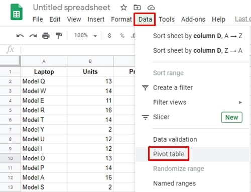
- Now, click on Data which should be in the menu bar at the top.
- From the pop-up menu, select Pivot Table.
- You will be asked if you wish to add the Pivot Table to the existing tab or if you want to add it to a new tab. Choose your preferred option and the table will be created.
- The new tab which should be named as ‘Pivot Table 1, 2, 3…’ and so on based on the number of Pivot Tables in the spreadsheet.
As you can see, creating a functional Pivot Table is as easy as it can be. And now, once you’ve created the Pivot Table you also might want to know how to edit the table to get different results from the dataset.
How to edit a Pivot Table in Google Sheets
As you create a Pivot Table, you will see the Pivot Table editor options show up towards the right side of the screen. From here, you will have access to all the editing options to tweak the Pivot Table. What’s even more interesting is that you can take advantage of Google’s advanced AI to generate your table.
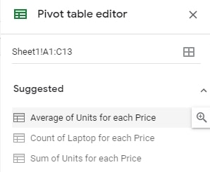
When you create a Pivot Table, you will see a few suggestions appear in the Pivot Table editor. These suggestions will vary based on the data in the table. If you click on a suggested Pivot Table, it will automatically organize all the data and give you the desired results. Although, this feature is not guaranteed to work with every dataset your throw at it. Nonetheless, you can also manually edit your table as well and we’ll be showing you how to do that below.
The first thing you will notice when you create a Pivot Table is these four options:
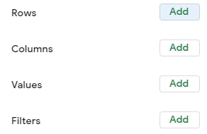
- Rows: When you add a row, it will give you the option to select one column heading from the list. And when you select a heading, all the unique items from that column will be added to your Pivot Table.
- Columns: Adding a column is somewhat similar to adding a row. Although, it adds the items/data in the top section of the table as columns. And you will be able to see the aggerated data of the selected columns.
- Values: The value option is fairly simple. When added, it will allow you to get the sum, average, or other quantitative results for the selected data. So basically, the Values option adds the value from the selected heading to the table.
- Filters: This lets you set parameters to only show data that meets the specified criteria.
When you add a Row, Column, or Value, you will also be able to change how you want to summarize the data. Additionally, you can choose between ascending or descending order.
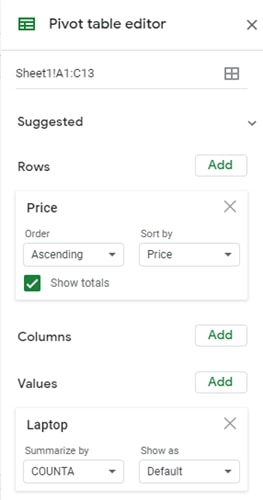
So in order to change these values, in the Row and Column options, click on the drop-down menu below the Order label. From here, you can select either ascending or descending order. As a bonus, you can even add a custom formula in the Values section. To do this, you need to click on Add (Values) and then click on Calculated Field. You will then need to input the formula that you wish to apply to the Pivot Table.
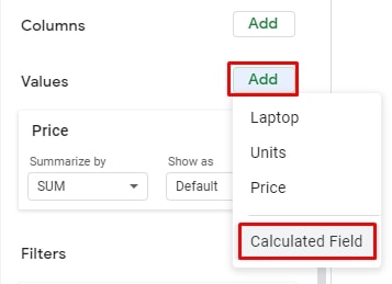
Alternatively, if you want to change the Value aggeration, click on the drop-down menu below the Summarize by label in the Values section. You will now see a list of functions that can be applied to give you the desired results.
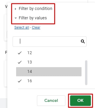
Coming to the Filters option, you can add a filter and then select which items you want to filter out from your results. This comes in handy to generate reports which require only specific details. After adding a filter, click on the drop-down menu below the Status label and select or deselect the items you want to add or remove from your Pivot Table.
Conclusion
Well, that pretty much sums up the basics of using the Pivot Table in Google Sheets. Understanding the working of the Pivot Table might take a couple of days. But once you become accustomed to using this handy tool in Google Sheets, you’ll never want to go back to using codes and functions.